Article #39: Parallel and Series
Operation of Pumps, and Operating against Multiple Systems
In most training exercises or general discussions of
pump-system interactions, great simplifications are made. The two most common
examples presented are usually two pumps operating in parallel, or two pumps
operating in series. Rarely, discussion involves more then two pumps, and even
less frequently operation of a single pump against a multi-branched system is
discussed. Yet, real installations rarely resemble such isolated and greatly
simplified situations. Usually, in practice, multiple pumps operate against
multiple branches of a system, or several interconnected complex systems
operated with pumps coming on and off line, valves adding multiple new
branches, or shutting off parts of the system.
Such multi-branched, multi-pump systems can no
longer be analyzed with a graph and calculator in hand, but an entire
computerized network of the plant piping, tanks, pumps, reflecting proper
sizes, friction, elevations, and so on, need to be carefully modeled.
However, before the complexities of the entire plant
modeling are attempted, the fundamentals of the multi-pump, multi-branch
systems must be first understood. When such examination is reviewed, it becomes
clear that the entire complex network is essentially a combination of the
following three cases:
- Several pumps in parallel, against a single system
- Several pumps in series, against a single system
- A single pump against two-branched system, or against a multi-branched
system
This article presents the fundamentals of such three
main building blocks of the complex network.
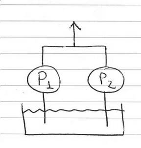
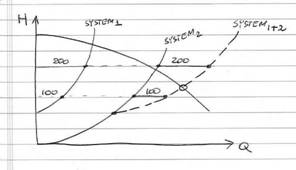
1-a: (2) pumps in parallel against (1)
system
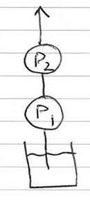
1-b: (2) pumps in series – against (1) system 1-c: (1) pump – against (2) system
branches
1-a: (2) pumps in parallel against (1)
system
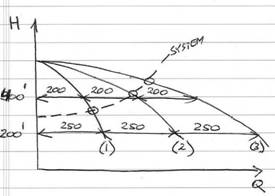
Method of
construction of multiple (combined) pump curve: at constant head line (200’)
double the flow (250 gpm x 2) for a point on a 2-pump curve. Repeat at several other
constant head lines, such as at 400’ double the flow (200 gpm x 2). For 3-pump
operation, triple the flow at constant head lines. Continue in the same fashion
for more pumps. Intersections between one, two, three, or more pumps, with a
given system curve establishes operating point (resultant head and flow) for
multiple pumps.
1-b: (2) (or more) pumps (or pump stages)
in series – against (1) system
Method of
construction of multiple (combined) pump curve: at series of constant flows,
add pump (or pump stages for multiple pumps) heads. Intersections between the
result pump curve (stages curve) and a system curves establishes operating
point (resultant head and flow).
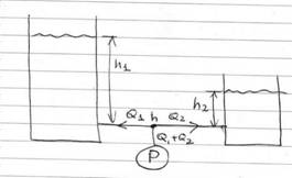
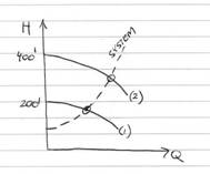
1-c: (1) pump – against (2) system branches
Method of construction:
instead of combining pump curves, add flows (at constant head) for systems (can
be more then two). Intersection of the resultant system curve with a given pump
curve produces operating point (resultant flow and head)
This process
can be computerized as illustrated in a simplified example of a positive
displacement pump operating against two systems (two branches). Underlying
programming formulas are:
(1) H = h1 +
k1 x Q12 – general equation for a system of
branch (1), including static head h1 and friction with system friction
resistance k1
(2) H = h2 +
k2 x Q22 – general equation for a system of
branch (2), including static head h2 and friction with system friction
resistance k2
(3) Q = Q1 +
Q2 – what leaves the pumps splits into branches
Known/given:
Q, k1, k2, h1, h2
Need to
find: Q1, Q2 and pump head h
Programming procedure:
- Guess h
- Calculate Q1 from (1)
- Calculate Q2 from (2)
- Calculate Q=Q1+Q2 and compare with given Q
- If calculated flow is different then given,
re-guess h and repeat the process until error is small
Click: 2-branched
system with 1-pump: sample
Only when these
fundamental basics of the pump(s)-to-system(s) principles are understood, you are
ready to take the next step – a computerized analysis of complex pumping
systems.